Algorithms Class Notes
Part 1
Question 1.
.png)
algorithm getCouples(M, W){
    Sort M in descending order
    Sort W in descending order

    i = 1
    j = 1
    while i <= n and j <= m {
        if M[i] < W[j] {
            j += 1
        }
        else if M[i] <= W[j] + 3 {
            pair up M[i] and W[j]
            i += 1
            j += 1
        }
        else, i += 1
    }
}
Let the array of man M = \([m_1,m_2,...m_n]\) and array of woman be \([w_1,w_2,...w_3]\) in sorted order.
Let us assume for the argument, that our solution pairs up \(m_1\) and \(w_1\).
Lemma : There exist an optimum that pairs up \(m_1\) with \(w_1\).
Let us assume that \(m_1\) is not paired with \(w_1\) in the optimum, while it is a valid pair.
Case 1 - Let us assume \(m_1\) is paired with \(w_n\) and \(w_1\) is unpaired in the optimum.
Now, we can swap \(w_n\) with \(w_1\), that is, \(Optimum - [m_1, w_n]+[m_1, w_1]\), which will not alter the number of pairs in the optimum.
Case 2 - Let us assume \(w_1\) is paired with \(m_n\) and \(m_1\) is unpaired in the optimum.
We can swap \(m_n\) with \(m_1\), that is, \(Optimum-[m_n, w_1]+[m_1, w_1]\), which will not alter the number of pairs in the optimum.
Case 3 - Let us assume \(m_1\) is paired with some \(w_j\) and \(w_1\) is paired with some \(m_i\).
Since, \([m_1, w_1]\) is a valid pair, then, we can confirm that \([m_i, w_j]\) is also a valid pair. Thus, by exchange argument, we can perform the operation, \(Optimum -[m_1, w_j]-[m_i, w_1]+[m_1, w_1]+[m_i, w_j]\), which will not alter the number of pairs in the optimum.
Thus, from exchange argument, our soultion is as good as the optimum.
Analysis of the running time
The running time of the algorithm is dominated by the sorting step, thus the running time is \(O(wlogw+mlogm)\) where w and m are the sizes for list of males and females.
Question 2.
.png)
algorithm getCredits(B){
    i = 1
    s = 0
    while i <= h{
        m = max between all B[i, j] for j in [1, n]
        s = s + m
    }
    return s
}
Let us consider our solution contains the element B[1, 1].
Lemma 1 : There exist an optimum which includes the entry B[1, 1]
Let us consider an optimum soultion for the problem which includes the entry B[1, t]. Now we can argue that B[1, t] cannot be greater than B[1,1], because if it were the case, then our algorithm should have chosen B[1, t] in its solution along all B[1, j] for all j in [1, n] for the first hour.
Thus the credit value for B[1, t] should be as good as B[1, 1]. Thus, B[1, 1] belongs to some optimum.
Now, Let us consider our solution contains the element B[a, b].
Lemma 2 : There exist an optimum which includes the entry B[a, b]
Let us consider an optimum soultion for the problem which includes the entry B[a, t]. Now we can argue that B[a, t] cannot be greater than B[a, b], because if it were the case, then our algorithm should have chosen B[a, t] in its solution along all B[a, j] for all j in [1,n] for the first hour.
Thus the credit value for B[a, t] should be as good as B[a,b]. Thus, B[a, b] belongs to some optimum.
Analysis of the running time
The loop takes nh time to execute, thus the running time for the algorithm is \(O(nh)\).
Question 3.
.png)
def removeMax(f){
    i = 2
    while i <= n-1{
        if f[i] is a local maximum {
            if(i+2<=n)
                then, f[i+1] = max(f[i], f[i+2])
            else f[i+1]=f[i]
        }
    }
    return f
}
Let us consider our solution alters the entry A[n] to A[c]
.png)
Lemma : The optimum alters the entry A[n] to A[c]
Case 1 - Let us assume the optimum does not alters the value of A[n].
In this case, to nullify the local maximum at A[b] and A[c], the optimum will have to perform 2 operations, that is A[b] to A[n] and A[c] to A[n]. This will take an extra operation. Thus, our initial assumption was wrong, the optimum have to alter the entry A[n].
Case 2 - Let us assume the optimum alters the value of A[n] but not to A[c].
Suppose the optimum alters the value of A[n] to T. if T \(\ge\) A[b] and T < A[c], then it will diminish the maximum at A[b], but it will need another operation at A[c]. And if T>A[c], still it will have to make another operation to counter the new peak at A[n].
Thus, our initial assumption was wrong. The optimum will have to alter the value of A[n] to A[c].
Case 1 and 2 proves the lemma.
Similarly, we can prove that for each change we make in the array, the optimum will have to make the exact change in the array. Thus our solution is as good as the optimum.
Analysis of the Running Time
The running time of the algorithm is dominated by the while loop, which takes \(O(n)\) time.
Question 4.
.png)
- I would disagree with the Candidate Greedy Strategy I, as this strategy may fail in certain situations. As an counter example,
Let as consider that we need to find machines for the spectrum range L=1 to H=12 and the available technologies \(T_1[1, 4]\) \(T_2[5, 8]\) \(T_3[9, 12]\) and \(T_4[2,7]\).
.png)
As per the Greedy Strategy I, the solution for the problem will be \([T_1T_2T_3T_4]\).
But for this problem, there exist a better solution for the problem, that is \([T_1T_2T_3]\).
This is because, the given Greedy Strategy will start with technology \(T_1\) since it covers the longest spectrum. But however, we can see, it comes out as redundent, as anyway, we have to have all the other technologies in order to cover the spectrum [L, H].
(b) I would agree with the Candidate Greedy Strategy II, and I believe the strategy always returns an optimum solution to the problem.
Let us consider that our soultion starts with the technology \(T_1\).
.png)
Lemma 1 : There exist an optimum that starts with \(T_1\)
Let us assume that there is some optimum that does not starts with \(T_1(l_1,h_1)\), rather it starts with \(T_n(l_n,h_n)\).
Now we can argue that \(h_n\) is always less than or equal to \(h_1\), this is because, if it were not the case, our algorithm shoud have chosen \(h_n\) over \(h_1\). Thus we can easily swap \(T_n\) with \(T_1\) and it will not allter the number of technologies in the soultion.
Lemma 2 : Our soultion is as good as the optimum
Let us assume our soultion as \([t_1t_2..t_n]\) while there exist an optimum as \([m_1m_2..m_n]\)
Consider the end range for an technology \(i\) as \(h(t_i)\) and \(h(m_i)\).
Case 1: \(i=1\)
From Lemma 1, we can assume the base case \((i=1)\) for this inductive proof, that is,
\(h(m_1)\le h(t_1)\) to be true.
Case 2: \(i=j\)
Let us assume, \(h(m_j)\le h(t_j)\) to be true
Case 3: \(i=j+1\)
We can argue that \(h(m_{j+1})\le h(t_{j+1})\) as if it were not the case, our algorithm must have taken \(h(m_{j+1})\) into consideration.
It proves that our solution is as good as the optimum.
Part 2
Question 1.

Solution Description
We will use the generic binary search algorithm. At every instance of the function call, we will check if the index of the Mid matches its value.
algorithm getElement(List, Base){
    Mid = List.size()/2
    if Base + Mid is equal to List[Mid], then return List[Mid]
    if List[Mid] > Mid + Base, then return getElement(List[:Mid], Base)
    else return getElement(List[Mid+1:], Base + Mid)
}

L = Input List
Result = getElement(L, 0)
Let k be the size of the input list.
Lemma: The algorithm returns the correct result for the list of size n.
Base Case : k = 1 Since there is only one element in the list, our algorithm just has to check if the value of this element is equal to its index (1 in this case) or not. Thus our algorithm returns the correct result for an input list of size k = 1.
Inductive hypothesis : As an inductive hypothesis, let us assume that our algorithm is correct for an input list of size k < n.
Inductive Step : k = n At each instance, our algorithm checks if the middle value of the list is our required answer.
If the value of the middle element = index of the middle element, then this is our answer. If the value of the middle element M > index of the middle element, then all the elements on the right side of M will surely not be the required answer. Thus we can discard this half and look for the result of the first half \([1,2,3,...\frac{n}{2}]\).
Similarly, if the value of the middle element < index of the middle element, we discard other half \([\frac{n}{2}+1, \frac{n}{2}+2, ... n]\).
In either case, the size of the subproblem is less than n; thus, by the induction hypothesis, we can say that the algorithm returns the correct solution for the subproblem.
This proves the lemma that the algorithm returns the correct result for the list of size n.
Analysis of the Running Time
At every iteration we are discarding half of the currently present elements from our search space. Thus, the recurrance relation for the algorithm can be given as
\(T(n) = T(\frac{n}{2}) + c\)
On solving the recurrance relation, we get, \(T(n) = O(log(n))\).
Question 2.

Solution Description
While searching for a \(k^{th}\) smallest element, we are sure that the element we are searching for is among A[i] and B[j] such that i + j = k. Thus initially, we will keep a pointer to the \(\frac{k}{2}^{th}\) element of both the arrays, and then we will compare the values of the pointed elements, based on which, at every level of recursion, we will discard half of either array from our scope of the solution.
algorithm getElement(A, B, k){
    if A.size() > B.size() then swap A and B
    if A.size() = 0 and B.size() > 0, then return B[k-1]
    if K = 1 then return min(A[0], B[0])
    i = min(A.size(), k//2)
    j = min(B.size(), k//2)
    if a[i-1] < B[j-1] then return getElement(A[i+1:], B, K-i)
    else return getElement(A, B[j+1:], K-j)
}
Let a and b be the size of the input lists.
Lemma: The algorithm returns the correct result for the problem of size m+n where m and n are the sizes of the input lists.
Base Case : a+b = 1
Since there is only one element in the list and the other list is empty, we can at max return the 1-th smallest element. Thus our algorithm returns the correct result for an input list of size a+b = 1.
Inductive hypothesis : As an inductive hypothesis, let us assume that our algorithm is correct for an input list of size a+b < m+n.
Inductive Step : a+b = m+n
We maintain two pointers i and j, for the lists A and B, such that i+j = k. At each instance, our algorithm checks if we have reached the k-th smallest element. If so, it returns us the result and halts it.
However, if it’s not the case, then it compares the value of \(A[i-1]\) and \(B[j-1]\), and based on it, it discards either \(A[:i]\) or \(B[:j]\) elements from our solution space.
In either case, the size of the subproblem is less than m+n, that is a+b<m+n; thus, by the induction hypothesis, we can say that the algorithm returns the correct solution for the subproblem.
This proves the lemma that the algorithm returns the correct result for the problem of size m+n where m and n are the sizes of the input lists.
Analysis of the Running Time
At any instance, we are discarding half of the elements from our search space from either list A or list B. Thus, the running time of the algorithm will come up to be as \(O(log(m)+log(n))\)
Question 3.
 Solution Description
For this problem, we would use the partition scheme of the quick select algorithm. In order to report the \(K\) nearest points to the origin, we will search for the \(K^{th}\) smallest point from the array. On finding the point, we can claim that all the points that are on the left of the Kth smallest point will surely be less than \(K\).
algorithm getPartition(P, L, H){
place P[L] at index i such that for all points t of P[:i],
dist(t) <= dist(P[i]) and for all points h of P[i+1:],
dist(h) > dist(P[i])
return i
}
algorithm getPoints(points, low, high, K){
if low <= high, then return points[:K]
p = getPartition(points, low, high)
if p = K then return points[:K]
if p < K then return getPoints(points, p+1, high, K)
else return getPoints(points, low, p-1, K)
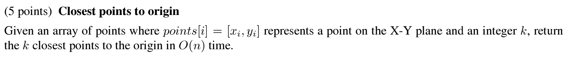
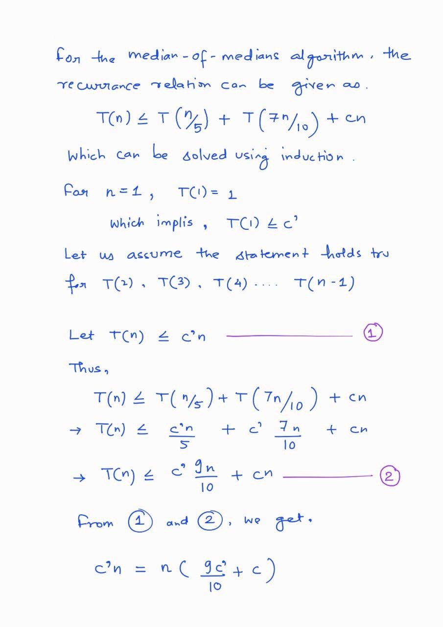
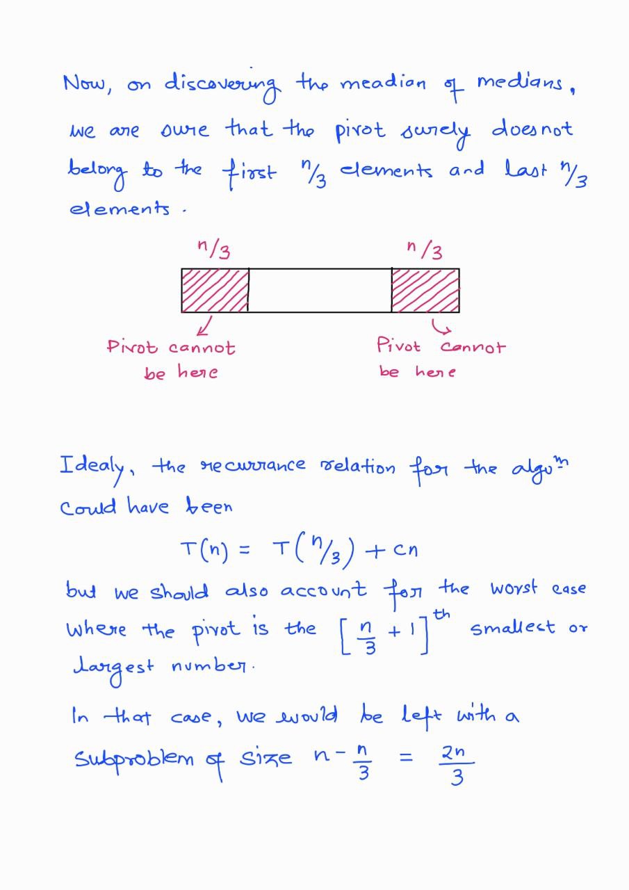
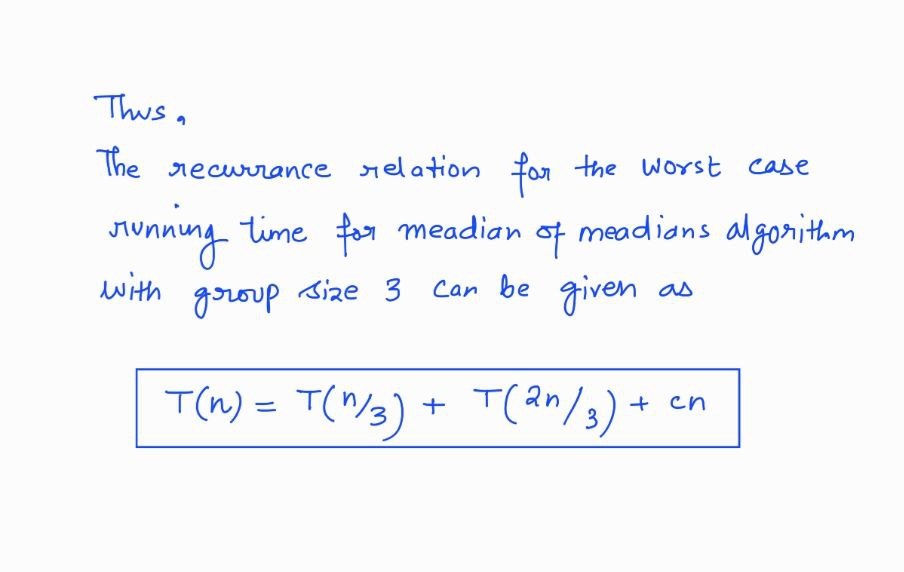
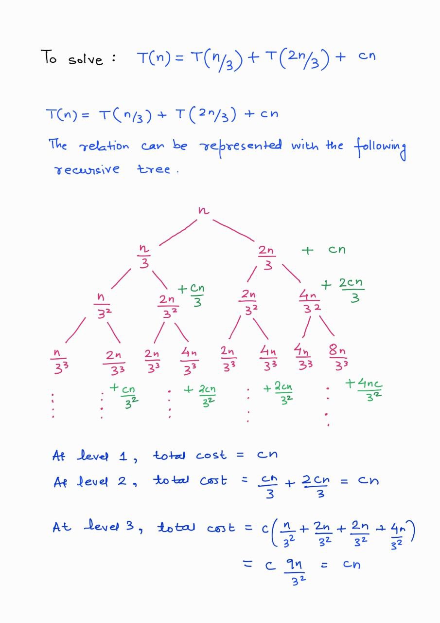
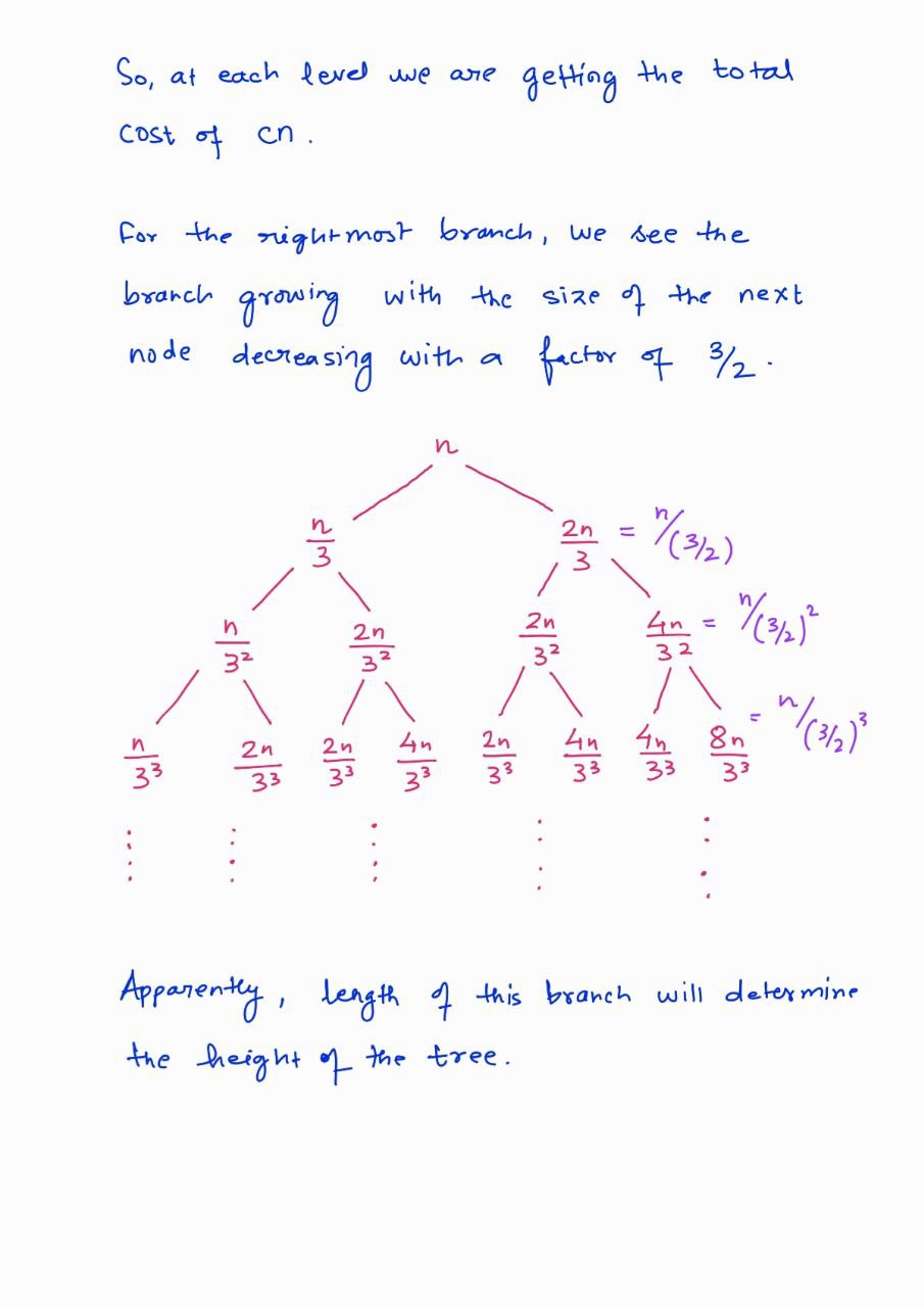
}Although the solution given above is correct and the time complexity at best case in \(O(n)\), but in the worst case it might go till \(O(n^2)\).
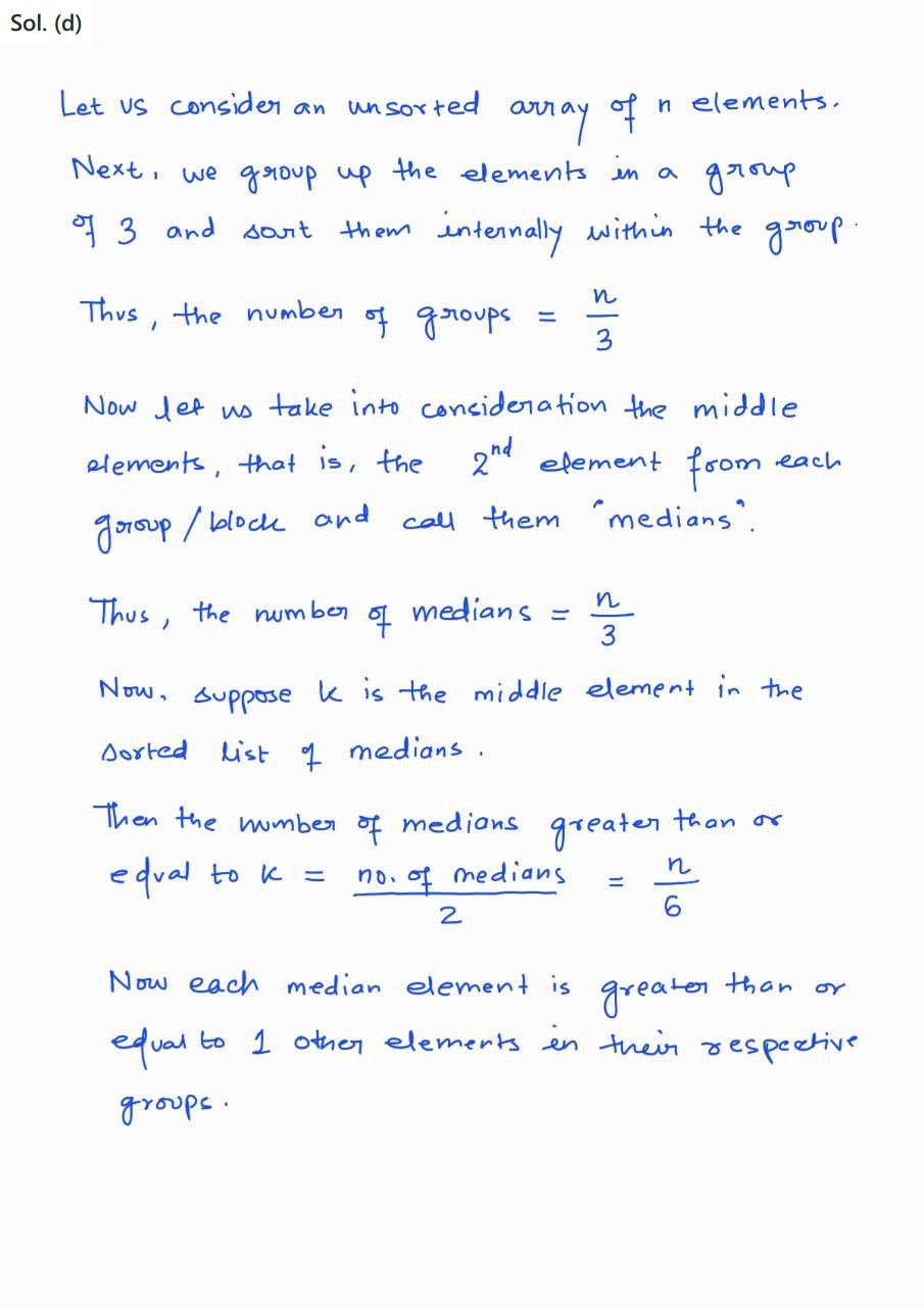
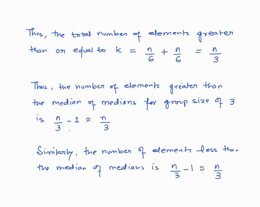
Thus, to ensure \(O(n)\) time complexity throughout, we can use a different strategy, which is based on median-of-medians.
algorithm getPartition(P, T){
    place P[T] at index i such that for all points t of P[:i],
        dist(t) <= dist(P[i]) and for all points h of P[i+1:],
        dist(h) > dist(P[i])
    return i
}

algorithm getPoints(P, L, H, K){
    divide P into groups of 5
    sort the groups internally

    middle = []
    for all a = middle elements of each group, do middle.append(a)

    if middle.size() is 1, then M = middle[0]
    otherwise, M = getPoints(middle, 0, middle.size(), middle.size()/2)

    pivot = getPartition(P, M)

    if pivot - L = K - 1, then return P[:pivot]
    if pivot - L > k - 1, then return getPoints(P, L, pivot - 1, K)
    otherwise, getPoints(P, pivot + 1, H, K - pivot + L - 1)
}
Let k be the size of the input list.
Lemma: The algorithm returns the correct result for the list of size n.
Base Case : k = 1 Since there is only one element in the list, our algorithm can at max can return the 1-st closest point to the origin, which in this case is trivial. Thus our algorithm returns the correct result for an input list of size k = 1.
Inductive hypothesis : As an inductive hypothesis, let us assume that our algorithm is correct for an input list of size k < n.
Inductive Step : k = n
At each instance, our algorithm checks if the middle value of the list is equal to K (since we are searching for K-th nearest point to the origin),
If the value of the middle element = K-1, then it returns P[: K-1] points where P is the list of the points. Otherwise, the algorithm compares the value of the middle element with K, and based on it, it either discards P[middle :] Or P[: middle] elements from our solution space.
In either case, the size of the subproblem is less than n; thus, by the induction hypothesis, we can say that the algorithm returns the correct solution for the subproblem.
This proves the lemma that the algorithm returns the correct result for the list of size n.
Analysis of the Running Time
The running time of the algorithm is dominated by the median-of-medians.
Question 4.
Part 3
Question 1.
Soultion Description
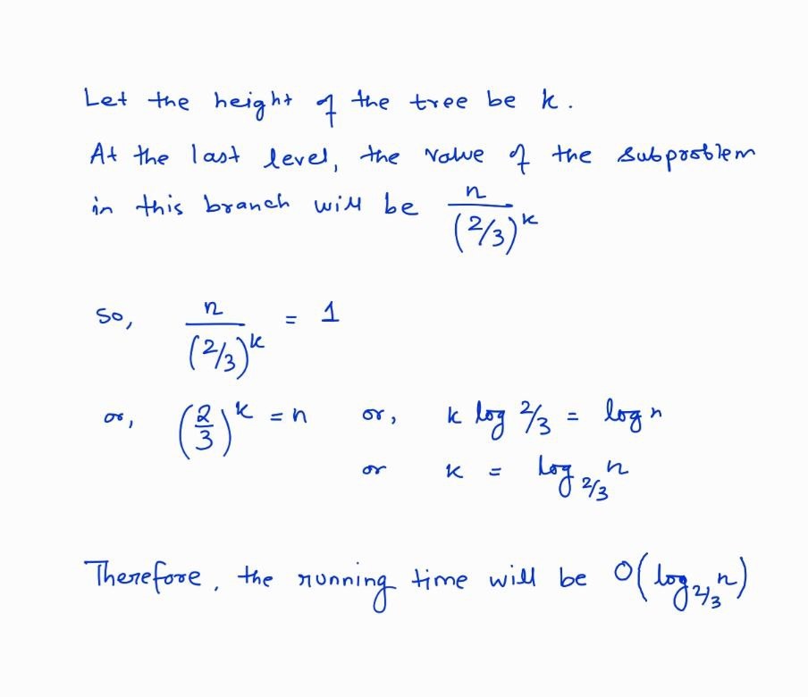
For a given array A[1..N] as input, we would maintain a buffer array B[1..N] where entry B[x] represents the maximum sum of the contiguous subsequence with A[x] as the last element of the subsequence.
B is a buffer array of size N
algorithm getMaxSubsequence(A[1..N]){
    B[1] = A[1]
    for i = 2 to N, do,
        B[i] = max(B[i-1] + A[i], A[i])
    index = index of the max entry of B
    if B[index] < 0:
        return []
    p = index
    while p >= 1 and B[p] >= 0, do p = p - 1
    return A[p+1..index]
}
The entry B[x] represents the maximum sum of the contiguous subsequence with A[x] as the last element of the subsequence.
Lemma - B[N] calculated by our algorithm is correct
Base Case : Entry B[1] is correct
The algorithm trivially returns the correct result for B[1]. This is because the max sum we can get as A[1] as the final element of the subarray is A[1].
Inductive Hypothesis : Let us assume that B[x] calculated by our algorithm is correct.
To prove : B[x+1] calculated by our algorithm is correct.
Since the entry B[x+1] depends upon B[x], and from our assumption, B[x] is correct, then the algorithm returns the correct entry for B[x+1].
The lemma, B[N] calculated by our algorithm is correct is proved.
Analysis of the running time
The running time of the algorithm is dominated by the loop which take \(O(N)\) time fo fill all the entriess in the buffer array. Thus the running time of the algorithm is \(O(N).\)
Question 2.
Solution Description
For finding the length of the longest palindromic subsequence, we will first reverse the input string \(X\), let it be \(X'\), and search for the longest common subsequence between \(X\) and \(X'\).
Now, for searching the longest common subsequence between the two stings, we would maintain a buffer array B[1..N, 1..N], where each entry in, say B[p, q] denotes the length of the longest common subsequence between the substrings \(X[1..p]\) and \(X'[1..q]\).
B[0..N, 0..N] is a buffer array of size N+1 by N+1
algorithm getMaxPalindrome(X[1..N]){
    X' = reverse(X)
    for i = 0 to N, do, B[i, 0] = B[0, i] = 0
    for i = 1 to N, do
        for j = 1 to N, do{
            if X[i] = X'[j], set B[i, j] = 1 + B[i-1, j-1]
            else, B[i, j] = max(B[i-1, j], B[i, j-1])
        }
    return B[N, N]
}
B[N, N] denotes the length of the longest common subsequence between X and X’ which is the length of the longest palindromic subsequence in X.
Lemma - B[N, N] calculated by our algorithm is correct
Base Case : B[1, 1] is correct.
The base case is trivially true. B[1, 1] = 1, if X[1] = X’[1], otherwise, B[1, 1] = 0.
Inductive Hypothesis : Let us assume the algorithm returns the correct result for all the entries B[\(i\leq x, j<y\)] and B[\(i< I , j\le y\)].
To Prove : B[x, y] calculated by the algorithm is correct.
Since, B[x, y] depends on the entries B[x-1, y-1], B[x-1, y], and B[x, y-1], which are correct as per our assumption; thus the algorithm calculates the correct result for the entry B[x, y].
Thus the lemma that B[N, N] calculated by the algorithm is correct is proved.
Analysis of the running time
The running time of the algorithm is dominated by the nested loops. Thus the running time of the algorithm is \(O(N^2)\).
Question 3.
Solution Description
For solving the problem, we will maintain a buffer array of size M by N, where the entry B[i, j] denotes the longest possible common substring with x[i] and y[j] as the last characters of the common substring.
B is a buffer array of size M by N
M = length of string x
N = length of string y

algorithm getMaxLength(x, y){
    maxLength = 0
    for i = 1 to M do
        for j = 1 to N do {
            if x[i] = y[j], set B[i, j] = B[i-1, j-1] + 1
            else, B[i, j] = 0

            maxLength = max(maxLength, B[i, j])
        }
    return maxLength
}
Lemma - B[p, q] calculated by the algorithm is correct
Base Case : Entry B[1, 1] is correct
The algorithm trivially returns the correct result for B[1, 1]. This is because, B[1, 1] will either be 0 if x[1] \(\neq\) y[1], and 1 if x[1] \(=\) y[1].
Inductive Hypothesis : Let us assume that the algorithm returns the correct solution for all B[1\(\leq\)(p-1), 1\(\leq\)(q-1)].
To prove : The algorithm returns correct result for the entry B[p, q]
Since the entry B[p, q] depends upon B[p-1, q-1], and from our assumption, B[p-1, q-1] is correct, then the algorithm returns the correct entry for B[p, q].
Thus, for all P in [1, M] and Q in [1, N], B[P, Q] is correct. The length of the longest possible substring is the max(B[1..M, 1..N]).
Analysis of the running time
The running time of the algorithm is dominated by the time required to fill up the entries in the buffer array B, which is of size M by N. Thus the running time of the algorithm is \(O(MN)\).
Question 4.
Solution Description
Given a bitmap A[1..M, 1..N] as input, we would create a buffer map B[1..M, 1..N] where entry B[a, b] represents a maximum area of a solid square block with B[a, b] as the bottom-right corner of the block.
B is a buffer array of size M by N

algorithm getMaxBlock(A[1..M, 1..N]){
   for i = 1 to M, do B[i, 1] = A[i, 1]
   for i = 1 to N, do B[1, i] = A[1, i]

   for i = 2 to M, do
      for j = 2 to N, do{
         if A[i, j] is 0, then set B[i, j] = 0
         else, set B[i, j] = min(B[i-1, j], B[i, j-1], B[i-1, j-1]) + 1
      }

   maxArea = 0
   for i = 1 to M, do
      for j = 1 to N, do
          maxArea = max(B[i,j], maxArea)

   return maxArea*maxArea
}
As entry B[i, j] represents the max solid block, with A[i, j] as the bottom right corner cell of the block.
Lemma - The algorithm return a correct result
Base Case : Entry B[1, 1] is correct
The algorithm trivially returns the correct solution. For a bitmap of size M by N, and with A[1, 1] as the bottom right corner cell, there are only two possibilities. That is B[1, 1] = 1, if A[1, 1] = 1, or B[1, 1] = 0 if A[1, 1] = 0.
Inductive Hypothesis : Let us assume the algorithm returns the correct result for all the entries B[\(i\leq x, j<y\)] and B[\(i<x, j\le y\)].
To Prove : The algorithm returns the correct solution for B[x, y].
Since, the max solid block possible with A[x, y] as the bottom right cell depends on the entries B[x-1, y-1], B[x-1, y], and B[x, y-1], which is correct as per our assumption; thus the algorithm returns the correct result for the entry B[x, y].
Thus, for all P in [1, M] and Q in [1, N], B[P, Q] is correct.
The max possible solid block is the max(B[1..M, 1..N]), and thus, the algorithm returns a correct result.
Analysis of the running time
The running time of the algorithm is dominated by the time required to fill up the entries in the buffer array B, which is of size M by N. Thus the running time of the algorithm is \(O(MN)\). Assuming \(M \thickapprox N\), the running time is \(O(N^2)\).